API

Loading COLMAP dataset

GaussianSplatting.jl supports datasets in binary COLMAP format. To load it, you specify which GPU backend to use and a path to the dataset root directory.

import GaussianSplatting as GPS

kab = GSP.gpu_backend()
dataset_path = "<path-to-colmap-dataset>"
dataset = GSP.ColmapDataset(kab, dataset_path;
    scale=4, train_test_split=0.9, permute=true)

• scale::Int = 1 controls the scale of images to load (usually between 1 an 8).
• train_test_split::Real = 0.8 train/test ratio split. E.g. 0.8 will select 80% of the data for training and 20% for testing.
• permute::Bool = true whether to shuffle data in a random order.

Dataset directory should have the following structure:

- sparse/0/cameras.bin
- sparse/0/images.bin
- sparse/0/points3D.bin
- images/

Additionally, if setting scale > 1, following directories should exist:

- images_<scale>/

Loading a RealityCapture dataset

Scenes aligned in RealityCapture / RealityScan are exported in a different shape, and have to be converted first:

- input/             the images, as exported
- camera-params.csv  the camera parameters, as exported
- points.ply         the point cloud, exported with XYZ & RGB

julia --project scripts/rc-convert.jl -s <path-to-rc-export> --resize

This writes images/ (plus images_2, images_4, images_8 with --resize) and a sparse/0/ COLMAP model in place, after which the directory loads with ColmapDataset like any other.

The conversion is not just a re-encoding of the poses. RealityCapture solves per-image intrinsics and lens distortion, while training expects one shared pinhole over undistorted images, so every image is resampled into a common pinhole. Two consequences are worth knowing about:

• The shared focal is raised until no image samples from outside its own frame, which crops the field of view slightly - the blank_pixels = 0 behaviour of colmap image_undistorter.
• Views whose focal deviates from the dataset median by more than --focal_tolerance (2% by default) are dropped, since a zoomed-in frame cannot be warped into the shared pinhole without leaving a black border that would then be trained against.

Images RealityCapture failed to register simply have no row in camera-params.csv and are ignored, as is anything else in input/. --max_points subsamples the initial point cloud, which is worth having because RC clouds tend to carry far-field background the cameras never approach.

Initializing Gaussians from dataset

Once you load the dataset, you can initialize Gaussian model from it by providing an array of points (means), their colors and scales.

gaussians = GSP.GaussianModel(
    dataset.points, dataset.colors, dataset.scales;
    max_sh_degree=3)

• max_sh_degree::Int = 3 set the maximum allowed spherical-harmonics degree. For a given degree d, each gaussian will have (d + 1)^2 color features. Set 0 to disable it. This will be used by during training to limit current spherical-harmonics degree.

Rendering Gaussians

To render Gaussians, we first need to initialize rasterizer on the given GPU backend:

kab = GSP.gpu_backend()
rasterizer = GSP.GaussianRasterizer(kab; width=1280, height=720, mode=:rgb)

• width::Int and height::Int control the rendering resolution of the rasterizer.
• mode::Symbol = :rgb set the rendering mode. Either :rgb or :rgbd (RGB + depth) is supported for now.

Once constructed, we can rasterize gaussians onto the image plane given camera that determines the position from which to render:

image_features = rasterizer(
    gaussians.points, gaussians.opacities, gaussians.scales,
    gaussians.rotations, gaussians.features_dc, gaussians.features_rest;
    camera, gaussians.sh_degree)

Depending on the mode, image_features will be either in 3xWxH shape (:rgb mode) or in 4xWxH (:rgbd mode).

We can save it to disk (first transferring it from GPU to host):

using FileIO, ImageIO

host_image_features = Array(image_features)
save("image.png", GSP.to_image(@view(host_image_features[1:3, :, :])))

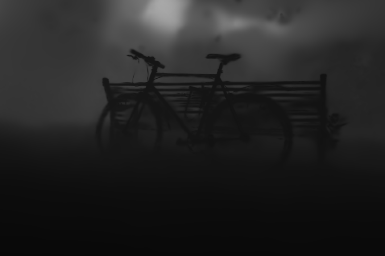
If the rasterizer is in :rgbd mode, we can also save the resulting depth map:

if rasterizer.mode == :rgbd
    depth_image = permutedims(@view(host_image_features[4, :, :]), (2, 1))
    depth_image ./= 50f0 # maximum(depth_image)
    clamp01!(depth_image)
    save("depth.png", colorview(Gray, depth_image))
end

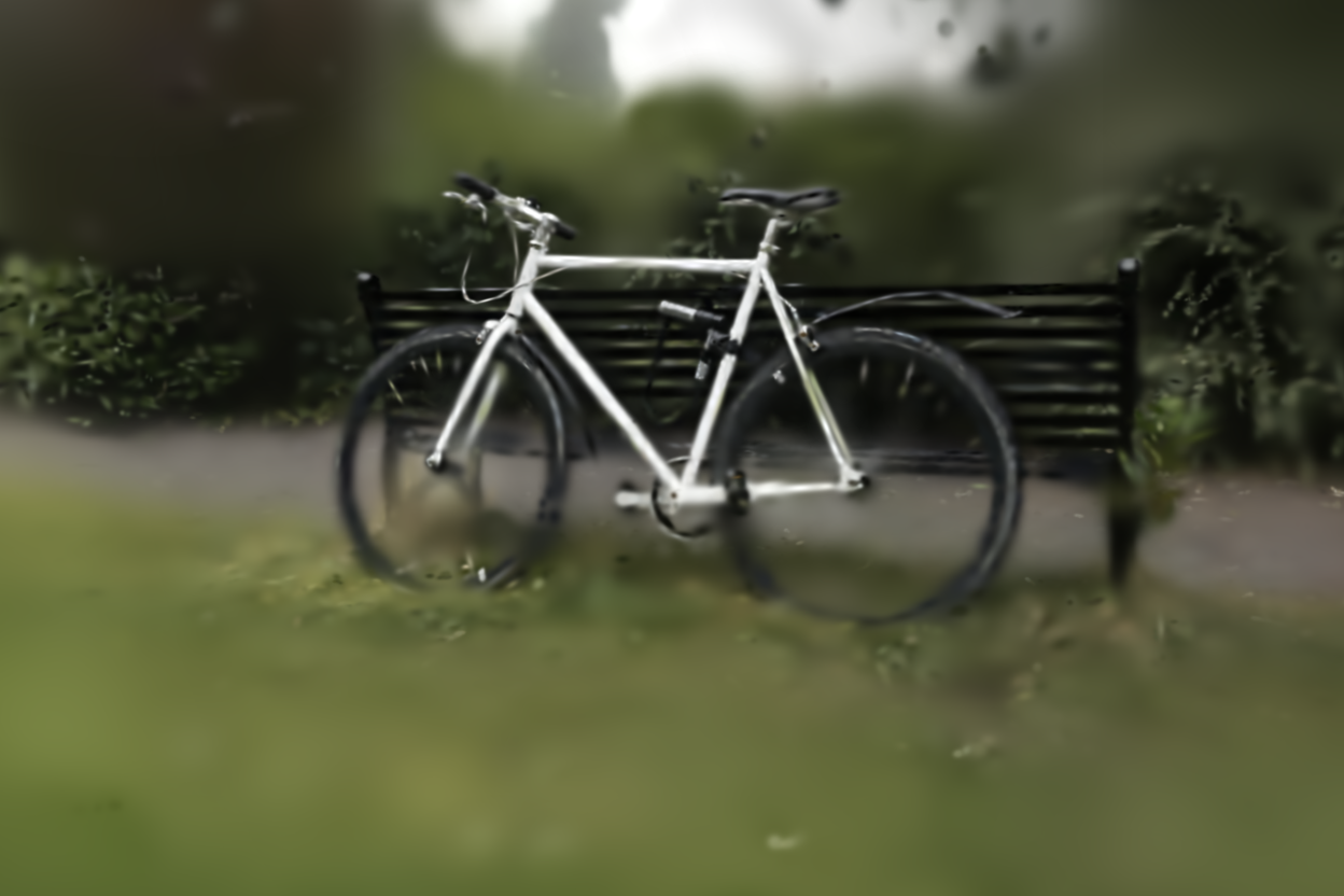
Example of rendering gaussians (bicycle dataset after 400 training steps):

RGB	Depth

Training Gaussians

GaussianSplatting.jl implements a Trainer that handles training routines such as loss computation, gradient update, model densification/pruning.

To construct a trainer pass:

• gaussians::GaussianModel that you want to train,
• rasterizer::GaussianRasterizer which it will use for rendering,
• dataset::ColmapDataset on which to train,
• opt_params::OptimizationParams that control learning rate (and its decay), densification and SSIM loss weighting.

opt_params = GSP.OptimizationParams() # Use default parameters.
trainer = GSP.Trainer(rasterizer, gaussians, dataset, opt_params)

To perform a single optimization step, just call step! on a trainer.

loss = step!(trainer)

If the dataset contains test data (e.g. train_test_split < 1), you can call validate to obtain validation metrics (SSIM, MSE, PSNR) accross test data:

(; eval_ssim, eval_mse, eval_psnr) = validate(trainer)